Six DoF Nonlinear Aircraft Model: Challenges in Software Development

Recently I wrote an article where I needed an aircraft model to simulate the phenomenon I was trying to describe. I’ve used a six-degrees-of-freedom (6 DoF) nonlinear model of an F-16 provided by the book Aircraft Control and Simulation (Stevens & Lewis, 2003). The codes were in Fortran and I translated them to Scilab scripts doing a little bit of software engineering and turn all of them into a small project at GitHub named McFlight. Through the next lines I will detail what is supposed to be a six-degrees-of-freedom nonlinear aircraft model, using the structure at McFlight as an example. And also I will try to assess how far (or close) such model is from the ones used by aerospace industry.

What is a 6 DoF Nonlinear Aircraft Model?

A very good approach to make science is to find a mathematical model to represent the piece of world you are interested in. Once your model is validated, you are able to make good predictions on that specific field. However, the beauty of a model is that you focus your spyglass on the relevant details of the observed phenomenon. For example, if I am studying the aerodynamics of wings, I would certainly be interested to model the flow detachment developing throughout the wing surface. But in a flight mechanics model I just need to know how aerodynamic forces change due to variables like angle-of-attack, Mach number, angle-of-sideslip, control surfaces deflections, regardless of how the flow detachment or any other specific aerodynamic phenomenon happens.

So we have an aircraft model to study the flight mechanics. This model is a set of ordinary differential equations and we may represent it as shown in Figure 1.

Figure 1. Differential equation for dynamic system model.

Basically we have a variable called state (X), a vector with the variables which describe the dynamics of our system, in this case, for example, we would have angle-of-attack, airspeed, pitch angle, rolling angle, sideslip angle, etc. And a variable called control (U) which represents the inputs in our system, in this case, the deflection of the aerodynamic surfaces (elevator, rudder, aileron, flaps, etc), engine setting or any other control input. Our model is the solution of the differential equations system shown in Figure 1. It is important to note that the input variables must be independent, otherwise it will be a state or output variable. The identification of the inputs is not always straightforward such that we have to be careful in order to avoid ending up with an incorrectly determined system of equations.

In mathematics, we say that a system is nonlinear when the output is not necessarily proportional to the input. For example, we cannot say that when we deflect the elevators, the lift force will increase by the same amount, differing only by a multiplication factor or that if we deflect the elevators in 5°, the increase in the lift force will correspond to the ones equivalent to 3° plus 2° deflections. In other words, the system will not necessarily respect the mathematical properties of linearity, which are:

• Additivity: f(a+b) = f(a) + f(b)
• Homogeneity: f(a*x) = a*f(x)

Nonlinear systems are much more representative of physical phenomena than linear systems. However, we have strong mathematical tools to work out on linear systems, including some of the most used design techniques for automatic control. Fortunately, we can link these two modeling approaches finding a linear approximation of a nonlinear model in the surroundings of an equilibrium point. Then we can make use of the linear mathematical tools, always paying attention to the assumptions taken on linearization process.

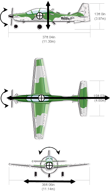
Finally, when we say six-degrees-of-freedom (or 6 DoF) we mean that our model is considering 3 translational and 3 rotational directions of movement as shown in the Figure 2 borrowed from this other article in which I discuss the “Aircraft diving before climbing or NMP zero in load factor response”.

Figure 2. Six degrees of freedom. The straight lines mean translational movements of back and forth following the arrows directions; the arches mean rotational movements clockwise and counter-clockwise around the center of gravity of the aircraft (assumed to be in the circle with the cross in the pictures). (Embraer super-tucano three views were found here).

Software requirements for the implementation

The main objective of the model we are describing here is to assess the flight mechanics and eventually to support the design of automatic flight controls. Then let us follow briefly a typical cycle for flight controls system (FCS) development so that we can tackle the main needs from a software engineering perspective.

Considering a classical approach, as stated by Rauw, the very first stage would be running (guess what) a 6 DoF nonlinear aircraft model starting from different trim conditions (equilibrium points, as explained below), mainly to get the feeling about the plant dynamics and aircraft mechanics as a whole. Also this nonlinear model will be the input for the linearization process which, in turn, will provide the linearized models for the controller design. Notice that both linearization and simulation operations will require a trim condition (provided by a trimming operation), but they are not related to each other. In other words, the linearization of the nonlinear model does not depend on the simulation of this model.

Breaking down the operations in further details:

• We need to trim the aircraft model. This means we have to find the inputs and states values to “balance” the plant, such that the states derivatives are equal to zero. Finding these equilibrium conditions can be done by building a cost function whose minimal value gives us a trim condition as a solution (this is a possible approach and the one we are using here);
• We need to run the model. This means solving numerically the differential equation representing the model (Figure 1), using the trim conditions found above to initialize the model;
• We need to linearize the model for different trim conditions. This means finding a first order approximation for the model function in the surrounding of a given equilibrium point. This will support the controller design (assuming we are using a linear design approach).

Trimming and running the model enable us to simulate (off-line, which means here that is not real time simulation as Rauw called) many conditions and maneuvers throughout the flight envelope, helping even to clarify the requirements for the controller itself. Also we will need to assess how to discretize the flight envelope for the controller design, which means choosing the points to linearize the model. But what we are interested to highlight here is that the activities listed above (mainly trimming and running), which use the nonlinear aircraft model, will be executed very often, so it is desirable that they can perform computationally as fast as possible. We don’t want to wait minutes to trim the model or that 1 second of off-line simulations run in 1 or more real second.

Once we finished the linear design of the controller (using linear analysis with robustness, comfort and some performance criteria) we have to keep going with the development adding the controller in the full nonlinear aircraft model “to ensure that the design works in this domain” (as shown in this GARTEUR book). Notice that we will have to take our designed linear controller to the nonlinear (more representative) full model, doing the necessary adaptations. And as taught by master McRuer, the next step “usually involves a series of increasingly realistic tests that attempt to thoroughly analyze the system in both normal and abnormal operating conditions”. This may imply the use of different test environments: from the real FCS software plugged into the nonlinear aircraft model to the “Iron bird” tests. We have to assure the equivalence between each test/development environment such that, in a final extent, we can be confident that the FCS eventually flying is the same designed on ground.

The development of an aircraft model is the result of a team work. We have propulsion data, aerodynamic data, mass distribution data, eventually we have to be aware about the sensors, the actuators and the dynamic modes of the structure, and any further data from other disciplines involved in the process. During the development these data will be iteratively updated. We have to be able to isolate these categories of data in our aircraft model such that we can quickly update each part separately and possibly add new parts.

Now hopefully we have a more clear picture of the main concerns when implementing our model:

• Performance. A software that runs quickly is always very welcomed. Throughout our design cycle we will need to run and re-run the model many times both in off-line or real time simulations, possibly in many different environments. But we have to be careful in how much performance we really need. We may waste too much time and efforts trying to improve code performance beyond our needs, risking to end up spoiling some other important code properties, such as readability. Although it is very difficult to figure out how much performance we will need in early stages of development, we can modularize the model so that we can improve the performance bottlenecks in later stages if it is necessary. Also, we can use different models in different environments (not all of them requires the same level of performance and mutability), but in this case we must have strong procedures to assure the equivalence between the models or, for example, trusted qualified tools to translate from one model to the others;
• Modularization. In software engineering history, we have an extensive list of reasons why you should modularize your code. In this specific case we can point out few but very strong justifications for doing so. We will have many people working in the same model at the same time, merging their work can be easier if they are changing separated modules. We will have parts of our model coming from other teams (possibly using different software tools) and we will also have to provide parts of our model to other teams; again, if we have well defined modules, this will be more efficiently done. And finally, as we stated in the previous item, if, for example, we find necessary to improve performance, this will be easier to change if we tackle specific modules of our model. Notice that most of the advantages of modularization comes from a very well defined interface between the modules, this means an interface that is very unlikely to change. For example, no matter how the aerodynamicists change their data and calculations internally, we will have our integrated model still working as long as their module keeps receiving alpha, beta, Mach, etc, as inputs, and providing the aerodynamic forces and coefficients as outputs;
• Readability. Once again, an aircraft model is a work of many hands. When caring about the readability, we reduce the amount of time required for the understanding of a given piece of code, even for the author of that code when looking at it again in the future. This also reduces the possibility of coding errors, making changes faster and safer. We talked so far about coding, but it is important to say that the widespread approach in industry for dynamic systems modeling is the model-based design which relies on its visual method to improve readability.

Implementation: McFlight architecture

As we explained previously, our McFlight is a possible implementation of the model provided by Stevens and Lewis. For further details about their model, please refer to the section 3.5 (Aircraft models for simulation) of the second edition (2003). Details about the equations will be found in the chapter 2 of this book. The implementation of the 6 DoF nonlinear F16 model is given by the authors using structured programming in Fortran, according to the following set of functions:

• Subroutine F: is the actual dynamic model containing the equations of motion, equivalent to the mathematical function f at Figure 1. This subroutine makes use of all the other functions below;
• Subroutine ADC: meaning airdata computer and responsible for the atmospheric calculations (mach, dynamic pressure, etc);
• Functions TGEAR, PDOT, RTAU and THRUST: responsible for the engine calculations;
• Functions for aerodynamic data: a set of functions representing the aerodynamic coefficients and forces.
• A cost function for trimming.

It is also provided some numerical algorithms for trimming, differential equation solving and linearizing.

Our (re)implementation of this model will try to pursuit the requirements described in the previous section. The high-level description is illustrated by the UML (Unified Modeling Language) diagram of components shown in Figure 3. For those not familiar with UML, this diagram aims to focus on the interfaces between the different parts of the software, each of these parts with a very well-defined concern (a component). The components are represented by a square with two small other squares on the left. The dotted-line arrow indicates a relation of dependency between the components, meaning that the origin depends on the destination. We also enclosed some components with similar concerns in what UML calls package (the square with an upper small square with a label). Notice that we are able to replace a component for another one with a different internal implementation but providing the same services to their dependent components, and keeping the whole system still working. In other words, as long as we keep the contract assumed between two components (the interface), they are transparently interchangeable by other ones implementing and using the same interfaces.

Figure 3. UML component diagram of McFlight.

We used Scilab scripts for the implementation and despite of not coding a canonical description of component (how it would be in Java, for example) our modules try to follow the same concept. In the following items we link the diagram at Figure 3 to the code at GitHub.

• Atmosphere (atmosphere/atmosphere.sci): model of the International Standard Atmosphere, providing temperature, pressure and density data based on altitude;
• Aerodata (eqm/aerodata_f16.sci): functions providing aerodynamic forces and coefficients data based on aircraft angles and control surfaces deflections;
• Engine (eqm/engine_f16.sci): functions providing engine thrust and dynamics based on throttle setting;
• Params (eqm/params_f16.sci): function returning geometric and mass properties of the aircraft;
• EQM (eqm/eqm.sci): actual implementation of the equations of motion of the aircraft, i.e., the function f represented in Figure 1. It requires the implementation of all components enclosed in the aircraft and nature packages shown in Figure 3.
• Trimmer (trim/trim_f16.sci): algorithms and functions for trimming the dynamic system represented by EQM;
• Simulator (sim/sim_f16.sci): algorithms and functions to solve the dynamic system represented by EQM, i.e., to run the flight simulation;
• Linearizer (sim/lin_f16.sci): algorithms and functions to find a linear model in a given trim condition.

I am not an advanced user of Scilab (yet) but I used two approaches to decouple the dependency between the modules (note: by “decoupling” here, we mean that the dependency relies on the well-defined interfaces as much as possible): (1) calling different .sci files which implement the functions with the same signature expected by the script (for example, in order to change the engine, wherever a file is executing engine_f16.sci on top, I could replace by, let’s say, engine_delorean.sci); or (2) passing a struct as a function parameter, assuring that it follows the expected data structure (for example, the parameter params in eqm.sci). If we succeeded in decoupling the modules implementations, we would be able to do things like, for example:

• Replace the module Aerodata for a newer version of aerodynamic data;
• Change the internal algorithms used by Trimmer, Simulator or Linearizer;
• Few changes enhancing the model to include sensors, actuators and a feedback controller;
• Replace the whole package Nature for other planet atmospheric model (and also gravity model which is currently tangled inside eqm and then not enough decoupled) enabling us to simulate our aircraft somewhere else in the universe;

As we said before, an alternative approach to implement dynamic models (and actually the de facto standard in aerospace industry) is the model-based design. We just want to make clear that it is possible to use this approach still keeping the decoupling philosophy behind the diagram at Figure 3. Indeed we are starting the equivalent implementation using Scilab Xcos.

To finish this section I would like to share a strategy in the methodology I followed when writing the scripts. For each module I developed, I tried to build a piece of automatic test. For example, for the atmospheric model, I wrote a CSV file with some data directly extracted from the NASA document of the standard atmosphere, and made a script to automatically compare each line of this CSV with the values returned by the implemented function (check the folder called tests). This reminds me what I heard from a senior engineer once: prior to any assigned task, figure out how you are going to validate it.

How far are we from the real world of the industry?

Imagine that you have decided to spend your fortune of billions of dollars developing an aircraft by your own or at least the FCS of an existing one. Would it be possible of doing so with the very simple application described above? Well, certainly our model would have to be enhanced. Let us infer what else we need when it comes to the real world of the industry.

• The data available would be massive. For example, the aerodynamic data would include the contribution of each surface in each different configuration of the aircraft, possibly in ice condition, throughout the whole flight envelope. One possible way to implement the nonlinear effects is using lookup tables and this certainly would give us thousand of tables to be interpolated. This means that we would have at least to include many other inputs to our aerodata module and be able to handle quickly the lookups in the tables;
• Care about the architecture trade-offs wisely. It is very beautiful to have a decoupled and componentized architecture but do not overengineer it. For example why would we isolate the codes related to atmosphere and gravity to the extreme if our aircraft surely will never fly in outer space? This can even compromise the software performance.
• Care about the software performance and ways to improve it when it is necessary. Being very specific, we shall always have means to compile our model or at least parts of it to make it faster, for example. As I said before, remember that we have to linearize around several points of the flight envelope and simulate before that, to check in what regions we should increase the number of points (transonic region, for instance) to improve our design.
• Eventually we will have to mix discrete and continuous time simulations. This means we would have to face all sort of problems with sampling, for example. The model-based design approach makes it easier.
• Have a robust version and configuration control of each module, or artifact. Eventually we will have to reproduce some simulation environments with different versions of engine, aerodata, mass properties, etc, for example. Having a rigorous tracking framework for our artifacts changes, helps us avoiding and fixing problems. Additionally this would make our lives easier when we need to talk to the aeronautics certification authorities.

Bad news (or good news) are that you won’t be able to make it by yourself. The pieces of information in each of the blocks in Figure 3 would be the result of many hours of work of many engineers. In the real world, the cherry on top of our challenge here would be the management effort to keep all the teams working synergically to achieve what was planned, constrained by the predicted time and budget. Piece of cake!

References

Magni, J.F., Bennani, S., Terlouw, J. (Eds.): Robust Flight Control: A Design

Challenge. Lecture Notes in Control and Information Services 224, Springer Ver-

lag, 1997.

McRuer, D., Ashkenas, I., Graham, D.: Aircraft Dynamics and Automatic Con-

trol. Princeton University Press, Princeton, New Jersey, USA, 1973.

Rauw, M. FDC 1.4 - A Simulink Toolbox for Flight Dynamics and Control Analysis.

Stevens, B.L., Lewis, F.L.: Aircraft Control and Simulation. John Wiley & Sons

Inc., 2003.

Aircraft diving before climbing or NMP zero in load factor response

Source: pixabay

Imagine a conventional aircraft, like the ones which are flying across the world carrying passengers, for example. There is a very subtle and intriguing fact (at least for flight mechanics geeks) when the aircraft is commanded “to climb up”: the very first response of the aircraft body, for a short time period, is in the other way round, i.e., it dives a very little bit before climbing up. This fact is well explained by the aeronautical engineering experts and I’ll try to build up this explanation throughout the following lines. I’m assuming the reader has only some Mechanics background in the beginning, but the last section will require some Control Theory background, once that we will try to illustrate this puzzling concept called Non-Minimum-Phase (NMP) zero.

What actually happens

Let us start picking up some facts very well explained by the giants (Stevens And Lewis, John Anderson, Robert Nelson, etc). A conventional aircraft, flying straight with no changes in its altitude, has wings with this magical shape such that, roughly speaking, the greater the angle between a centerline through the wing section and the wind direction (called angle-of-attack), the greater the magnitude of the supernatural force upwards, called lift (Figure 1). The basics of the aircraft longitudinal commands (upwards and downwards) will be provided by the balance of the forces generated by the main wing and the horizontal stabilizer (little wing at the rear of the fuselage). More specifically, the longitudinal dynamics of the aircraft will be performed by the elevators, the small moving surfaces at the rear of the horizontal stabilizer. Moving up or down (both left and right simultaneously), the elevators are able to vary the vertical forces on the horizontal stabilizer making the aircraft climb or dive in a short term (assuming constant the other aircraft commands inputs) (Figure 2). 

Figure 1. Angle-of-attack and lift force, assuming straight level flight.

Figure 2. Elevator commands and longitudinal dynamics. Left sketch: elevators up, force in horizontal stabilizer downwards, counter-clockwise momentum, nose-up movement; right sketch: elevators down, force in horizontal stabilizer upwards, clockwise momentum, nose-down movement.

Considering our aircraft, flying straight and steadily with constant speed and altitude, if the elevators are moved upwards, we have the following sequence of events:

1. The final elevators position causes a decrease in the lift force on the horizontal stabilizer. The force vector can even possibly turn to downward sense;
2. The overall lift force acting in the aircraft decreases and the weight now is greater than the lift force, making the whole body accelerate downwards;
3. The variation of the force in the tail generates an angular momentum, resulting in a pitching up movement (aircraft nose up);
4. The nose up movement increases the angle-of-attack of the wing and therefore the lift on the wing;
5. The angular momentum variation due to the new angle-of-attack of the wing counteracts the momentum variation due to the vertical force on the stabilizer, eventually breaking the pitching up movement;
6. The increase in the lift on the wing is greater than the decrease in the lift on the horizontal stabilizer such that the overall lift force results greater than the weight, making the whole body finally accelerate upwards.

This sequence of events is assuming a time frame of few seconds after the elevators command, because in a long term, the aircraft will decelerate and require other input commands to restore the equilibrium condition or to settle in a new one.

But notice that the very first dynamic response of the aircraft (described by item 2) is in the opposite sense of the intended response, which is increasing the overall lift force of the aircraft. And so far we have a hypothesis. We need a model to confirm our suspicion and to dig into the details a bit deeper.

We need a model

Making science is not an easy job, neither is it cheap. So let’s trust the giants Stevens and Lewis and borrow their F-16 model. Just considering the hours of wind tunnel tests, the hours of engineering work compiling the aerodynamic data and the hours of real flight to validate the data make the costs go beyond the hundreds of thousands of US dollars (the hourly operating costs of the F-16 is around US$ 8,000). Luckily to me it only costs few days translating the Fortran code to Scilab and typing the aerodynamic data to the computer. I made the code available at GitHub, named mcflight.

Our model is a dynamic representation of an aircraft able to move in so-called 6 degrees of freedom (shortly 6 DOF): roughly speaking, 3 translational and 3 rotational movement possibilities (Figure 3). Although, for the simulation we are interested in, we only need 3 degrees of freedom, once that we are dealing only with longitudinal axis (i.e., translational movements upward/downward and backward/forward, and rotational movement of aircraft nose up/down).

Figure 3. Six degrees of freedom. The straight lines mean translational movements of back and forth following the arrows directions; the arches mean rotational movements clockwise and counter-clockwise around the center of gravity of the aircraft (assumed to be in the circle with the cross in the pictures). (Embraer super-tucano three views were found here).

By dynamic representation we mean a set of differential equations whose solution will provide us with the description of the aircraft movement throughout the time (for a very detailed explanation about the equations please check chapter 2 of Stevens and Lewis). In order to validate our hypothesis, we will need to “make” the aircraft fly steadily (wings level, straight flight) and then apply a small deflection on elevators to make the nose up. If we are right, we will observe a small decrease in lift force before building up.

To observe the lift force, in flight mechanics we use a physical quantity called load factor which is simply the ratio between the Lift force and the Weight (Figure 4). Although it is dimensionless, we express the load factor in g (referring to acceleration of gravity) and it can be positive, when Lift is in upward sense, or negative, otherwise. A very good g-meter is our stomach and you probably have experienced some g’s (positive) when riding a roller coaster. When an aircraft is flying straight and you are indulging yourself with a hot beverage served by the flight attendant, the load factor is 1 g (i.e. weight equals to lift) at that moment. During a normal airline flight you will experience slight variations around 1g, but the load factor will always be greater than 0. The negative g’s are experienced in aerobatic flights, for example, and notice that it is not only a simply free fall (which would be 0 g) but an acceleration downwards.

Figure 4. Load factor. Ratio between Lift Force and Weight.

Finally simulating

We are going to run a set of scilab scripts, analyze the time history of some variables (such as load factor) and use a lot of imagination to see an F-16 flying around.

The first step is to put our aircraft in a steady flight condition, which in our case means finding the elevator deflection and throttle setting (i.e., thrust provided by the engines) to allow a flight at constant speed, constant altitude, constant angle-of-attack. In other words, this is an equilibrium condition. The translation of this problem to our physical model is finding the solution of the differential equation using the proper set of constraints. In Aeronautics this is called trimming the aircraft. So let’s trim the aircraft in straight flight with wings level at sea level (altitude 0 ft) and with a speed of 200 ft/s. Asking scilab to solve it for us, we find the condition shown in Figure 5.

Altitude (h): 0 ft (sea level)
Speed (V): 200 ft/s
Throttle setting (engine): 0.287 (from 0 to 1)
Elevator deflection: 0.72° (-25.00° to 25.00°)
Angle-of-attack (alpha): 19.70º
Figure 5. Trim condition.

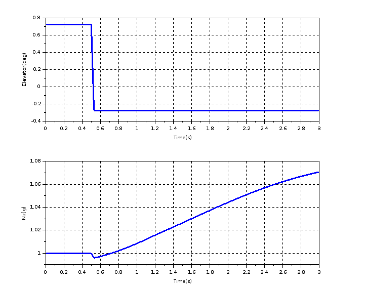
Let’s then apply the elevator deflection. In a time history simulation, we can say that it is a good practice to leave the aircraft fly steadily for a fraction of second (at least) just to check if there is an equilibrium point, before applying the input change. The following curves will show a time frame of 3 seconds of flight simulation with an elevator deflection of -1°, applied from 0.50s to 0.53s.

Figure 6. Load factor (Nz) and elevator deflection curves.

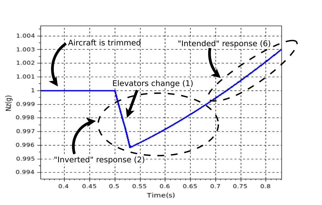
As we expected, the first dynamic response of the elevator deflection is a decrease in Nz. Then (after 0.53s) there is a monotonic increase in Nz until the end of the simulation. The Figure 7 shows the correspondence of the explained items in the previous section and the moments in the simulation zoomed in the first second of simulation.

Figure 7. Nz response right after elevator deflection. The numbers in parentheses indicate the corresponding item of explanation in the first section.

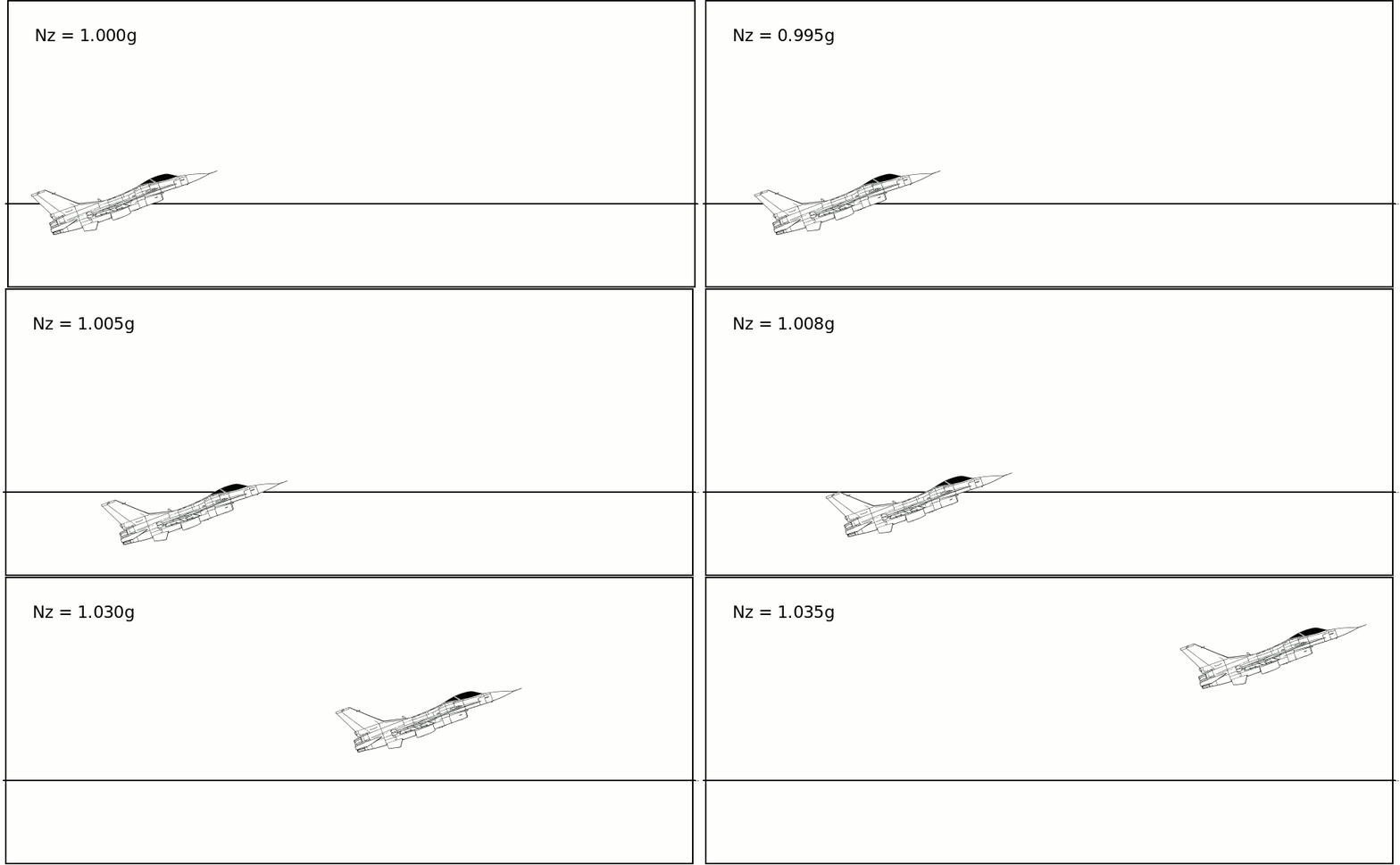
Notice that the amount of variation of Nz is around 0.004g, decreasing from 1.000g to 0.996g and increasing back in less 0.2s. This would be probable unperceivable by someone in the aircraft. A fighter like the F-16 is designed to be agile, to have a very fast dynamic response. If we had a model of a bigger guy (a cargo aircraft, for instance), the variation of Nz certainly would be slower and with a bigger magnitude (hopefully we will have another aircraft model available at mcflight soon). Figure 8 shows an illustrative animation of the F-16 flight.

Figure 8. Simulation F-16 model. Notice that the animation illustrates the drop in altitude, which is not coincident with the drop in Nz in the events timeline. Also the drop in altitude was (very) exaggerated for matters of illustration.

We could play with some parameters of our aircraft model to artificially make it have a behaviour similar to the bigger aircrafts. For example, we could change its ability to spin around the axis of the wings, i.e., the ability to nose up or down. Physically this means changing the moment of inertia around this axis. Try this out with mcflight code, varying the value of AYY.

From a Control Theory Point of View

From now on, it will be necessary some Control Theory background to fully understand it. A brave reader can keep going without this.

Considering the trim condition described in the previous section, we performed a linearization in order to find the state-space representation (Figure 9). In our Scilab scripts, this means using the command lin to find the matrices A, B, C and D and syslin to build a Scilab state-space representation. Mathematically we are reducing our flight dynamics to a first-order linear system representation of the equations. This will allow us to use the very well established theory of linear systems but the drawback is that this simplification is only compatible with the original (non-linear) model in the surroundings of the trim condition. So, before doing anything, we have to check the matching between our linear and non-linear models.

Figure 9. State-space representation, where x is the state variables vector, u is the control variables vector and y is the output variables vector.

Our linear representation is assuming the following variables:

• Control variables (u): throttle setting (engines) and elevator deflection;
• State variables (x): air-speed (assume that this equals to aircraft speed), angle-of-attack (alpha), attitude angle (theta, angle related to the horizon, initially equals to alpha), altitude, engine power setting.
• Output variables (y): load factor (Nz). 

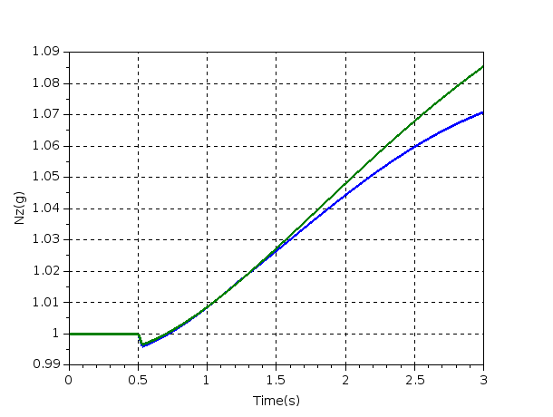
We can now simulate our linear model (in Scilab we can use csim command) with the same input we used in the previous section, using as input only elevator deflection and watching only the Nz as output. Figure 10 shows an overplot of linear and non-linear responses of Nz. Notice that after 1.4s our linear model starts drifting away from the non-linear model. However, the time frame from 0.0s to 1.4s is enough for our purposes.

Figure 10. Comparison between linear and non-linear simulations.

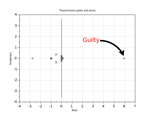
We are now ready to take a look on the poles and zeros of the transfer function of the system elevator-to-nz (Figure 10). Notice that we have a zero in the right-half-plane, also known as non-minimum-phase (NMP) zero (actually, we have three positive zeros, but the ones nearby the origin are due to the fact we inserted altitude and engine power as states, you can check this, eliminating them as state variables). And this guy is the guilty of the phenomenon we are describing here as stated by Stevens and Lewis (again): “these types of zeros occur when there are two or more different paths to the system output, or two or more different physical mechanisms, producing competing output components”. Yes, we have horizontal stabilizer and wings producing lift and affecting the load factor.

Figure 11. Poles and zeros of linear system elevator-to-nz.

Well, next time you are in a straight level flight of an airliner and all of a sudden you feel a quick and slight “floating” out of your seat (Nz less than 1g) before “sticking” to it (Nz greater than 1g) when the aircraft starts climbing, you can tell the passenger at your side that such sequence of events was caused by an NMP zero in the plant. Actually this is very unlikely, unless you have a g-meter with you. Anyway, at least the explanation you know ;-)

Why should I learn programming?

During every aircraft development, in order to assure that the flying machine behaves exactly as it was designed for, the flight test is performed by the manufacturer, also to prove to the competent authorities that the aircraft is able to fly safely. For the flight test purposes, the aircraft is equipped with all sorted of sensors (let’s say around 100,000 parameters), whose measured data we could assume recorded each 10 milisseconds. Doing a rough calculation we conclude that a single hour of flight test produces around 270 Gigabytes of data (in real life is actually much more than that).

The main point here is that for a single flight, there is a huge amount of data available to the aeronautical engineers validate and improve their design. But this only can happen in a phase of data analysis, which comes after few steps of processing the raw data, obviously unthinkable without some programming work. In a worst case scenario, the aeronautical engineers with their skills provided by a semester-long course of structured programming will struggle to write a little script from scratch to process the data and to allow them to check (for the thousandth time) if the aircraft behaved as expected.

This is not an isolated case of aeronautical engineering. Nowadays, in any field of science or engineering, our capacity to generate data has increased dramatically. For instance, the European Organization of Nuclear Research (CERN) announced (already in 2013) that their data centre had 100 petabytes of stored data, “equivalent 700 years of full HD-quality movies”. And the amount of general data produced daily is even more impressive. In every minute YouTube users share 400 hours of new videos, Facebook users share 216,302 photos, Instagram users like 2,430,555 posts.

This tells us that a problem-solving in this world overwhelmed by data is more and more walking towards formulate the problem for the computer helping us to solve it, no matter the field of knowledge we are talking about. This requires knowing how to ask the machine to solve our problem. As stated by an important Brazilian researcher, “every science is a computer science”.

Computer Science gap in other Sciences/Engineerings

If we compare a programming course in a standard engineering graduation today and 30 years ago, we would be impressed how topics are pretty much the same, sometimes only replacing Fortran by C, Python or even Matlab. Of course the basics of algorithms and problem-solving is very important to be kept, but the new engineers should at least be aware of the newest capabilities of programming and even the tools and techniques supporting the programming activity.

Resuming our example in the beginning of this text, aeronautical engineers 20 years ago could handle well (or, let’s say, using cutting edge technology by that time) the data available with their piece of Fortran code. Today, after getting (with a couple of clicks) the hundreds of gigabytes of data to analyze, they write a piece of code not that different than the one 20 years ago (in a different language, hopefully), but that runs in a hardware brutally faster and eventually achieve the expected results. Certainly, their job could be done faster by improving the code or by some different problem-solving technique; or perhaps many small repetitive tasks in the middle could be automated.

We could summarize this scenario as follows: in one hand we have engineers that eventually can make their job done, but is not fully aware that it could be improved by the latest programming capabilities available; on the other hand, we have computer engineers able to apply the best techniques but not required to help the other (non-computer) engineers.

Here we plotted the issue in the engineering field that is certainly far from being the worst case scenario, once that, at least, they have a programming course as part of their graduation. If we think about Human and Health sciences, the computer science gap may be much bigger.

Coding at School

Some people believe that in order to get over the aforementioned gap, we should go further and teach programming and related computer science topics earlier, at basic school. Hadi Partovi, the CEO of Code.org (a non-profit organization that aims expanding the access to computer science) said that “we don’t teach biology or chemistry to kids because they’re going to become surgeons or chemists, we teach them about photosynthesis and that water is H2O, or how lightbulbs work, just to understand the world around us. You don’t use any of it, but you do on a day-to-day basis use public-key encryption, and the average American has absolutely no idea what that is” (full text).

Besides initiatives as Code.org, programming contests worldwide has been becoming popular among youngsters before grad schools. The Brazilian Computer Society, for example, since 2002, offers modalities even for students under high school. The students shall solve computing and logical reasoning problems using just pencil and paper and, according to the Society, the goal is “to awaken the interest in computing problems and discover potential talents to programming”. The students with the best results in Brazilian Olympiad in Informatics will represent the country in the International Olympiad in Informatics which started at 1989 with 46 contestants from 13 countries and in its latest edition (2016) had 308 contestants from 80 countries.

Many countries have already included programming or “computational thinking” in their elementary school curricula. At European Union, 15 countries made it. And, at least in Brazil, where programming is not yet at the young students curriculum, private schools for “programming and robotics for teens” are rising in great cities like São Paulo, picturing a similar phenomenon which happened many years ago with the english private schools created all over the country. Sounds like the world is requiring the kids to learn a new language.

What about the future?

Studies published at the World Economic Forum Annual Meeting last year (2016) pointed some interesting facts about the jobs of the future: "The study shows that workers who successfully combine mathematical and interpersonal skills in the knowledge-based economies of the future should find many rewarding and lucrative opportunities."

If you realise that you can describe the routine of your day-to-day job in repetitive and well defined steps to execute some task, trust me, a computer program can do it way better than you can. This may sound alarming, but I can assure you that a significant percentage of a standard day at work of even very specialized science/engineering fields are covered by very repetitive tasks.

If at this point you are not convinced that you should improve your computational thinking skills, I quote the disturbing statement of this Brazilian researcher: “at this very moment, someone in the world is programming your job”.

Pragmatism doesn't mean reckless trial-and-error

When I finished my studies at university, I was eager to apply my technical knowledge in a real life context. And I confess that the very first contact with the crazy pace of job market was a bit shocking. At the time, as a purist, I incorrectly thought that using a pragmatic approach to solve a problem was akin to being reckless or irresponsible, which could only result in providing a sub-optimal solution. Later with experience it was eventually discovered that by wisely discarding parts of my theoretical knowledge it was possible to arrive more quickly at simpler solutions, without necessarily losing robustness.

According to Oxford dictionary, a purist is “a person who insists on absolute adherence to traditional rules or structures”. Also, it defines pragmatist as “a person who is guided more by practical considerations than by ideals”. This text intends to show that a purist approach can be relaxed and “more practically guided” still delivering successful solutions. This will be illustrated by a few examples in software and engineering contexts, but the technical details will be presented as lightly as possible so the reader from other fields can apply the examples to their own situations.

Would Physics equations from 1687 to 1905 be wrong?

In 1905, Albert Einstein proposed the ideas of his Special Theory of Relativity by the paper “On the Electrodynamics of Moving Bodies”, which pointed out some inconsistencies in Newtonian mechanics (1687) when speed approaches a significant fraction of the speed of light. Again, when the speed of the moving body is a significant fraction of the speed of light. Aircraft, for example, were (and still are) built using pure Newtonian physics with a successful history that speaks by itself. And how come, if these equations are not with the best precision? Well, Special Theory of Relativity adds a precision that is not required whatsoever by the models used for flying machines design. To give us an idea, the fastest speed ever attained by humans (11,1 km/s by Apollo 10 astronauts) will make Newtonian equations differ from Einstein equations by a factor of 0.9999999993 (being 1.0 corresponding to an identical result from both theories).

This bit of history helps us to illustrate how science works or more specifically how the scientific method works. When observing the problem we are interested to solve, we develop mathematical models, which are approximations of the natural phenomenon we are studying. The quality of a model in guiding us towards a solution will be determined by the degree of precision required in our solution. In other words, if our moving body speed is an insignificant fraction of the speed of light, we don’t need the degree of correctness provided by the Special Relativity Theory.

On the other hand our well-known Global Positioning System (also known as GPS) makes an elegant and crucial use of relativity theories to guarantee its very accurate precision, showing that each context dictates the required level of detail in the theoretical model.

What if aircraft were designed by the best purists in each discipline?

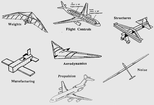
The concept and development of these amazing machines, weighing sometimes hundreds of tons, flying away from the ground and crossing oceans in a few hours, is the result of the hard work of thousands of people in several different disciplines. To enumerate just a part of them: aerodynamics, structures, flight controls, propulsion, electrical systems, hydraulic systems, etc.
If each of these disciplines worked strictly to attain their own requirements, we would have aircraft like the ones shown in the picture below, and none of them would fulfil all the requirements of the product at the same time.

As you can imagine, aircraft design is a huge effort of tuning the needs of all the disciplines together in one single product. And this has been working successfully for more than a century now.



Source: The Aerospace Design Process. A note from a reviewer friend: "I would prefer to see the glider associated with the aerodynamics and a parachute associated with noise" (Cap. Kev)

A bright tool called Object Oriented Programming (OOP)

The Object Oriented Programming (or shortly OOP), roughly speaking, is a way of programming such that the world is modelled by the concept of “objects”. An object encapsulates data (through the “attributes” concept) and the operations allowed over this data (through the “methods” concept). This paradigm, among many other features, allows the program to evolve and to be maintained more smoothly, using concepts like data encapsulation and code re-use, for example.

As far as I know, there is no hard, formal, mathematical definition for OOP (or any other programming paradigm), such that we say a programming language has more or less OOP features. Once I heard from a co-worker “if there is no explicit private/public keywords in Python, then it is not an object-oriented language”. By then, I started to think how an extreme purist view can make one blind. What are the questions we are really interested in answering? (1) Do we need an object-oriented language? or (2) do we need a software easy to be maintained and to evolve? I can assure you that is perfectly acceptable to use a multi-paradigm language that is not fully object-oriented but fulfil nicely your requirements. On the contrary, doing so, means studying carefully all the extent of your problem and then proposing a solution and not the other way round, i.e., picking up one solution and trying to make it fit to your problem.

For instance, if you have assessed all the main risks of your project, all the main test case scenarios (including the very critical ones) and mapped them in your development process, it really doesn’t matter what language or paradigm you are supposed to use. Unless your customer has a weird requirement that says you have to use a language with an explicit private/public keyword, you can use whatever your team is comfortable with. I would not be impressed with a very well written pure C code, implementing objects (yes, try to use function pointers into your structs and have fun).

The emerging agile philosophy all around

In this very well-written comparison between purists and pragmatist approaches, the BreakingSmart makes an enlightening statement about the agile philosophy: “today, the then-minority tradition of pragmatic hacking has matured into agile development, the dominant modern approach for making software. But the significance of this bit of history goes beyond the Internet. Increasingly, the pragmatic, agile approach to building things has spread to other kinds of engineering and beyond, to business and politics” (learn more).

Once the trial-and-error approach got the cost of a click on a computer, followed by results a few seconds later on the screen, hands-on creativity could walk along with productivity. But this triggers the uncle Ben’s warning: “with great power there must also come great responsibility”. It hasn’t been rare to hear that the agile methodologies are these magical tools which will make any development fit on any schedule. This is tricky and may possibly drive to an erratic trial-and-error approach without a minimal of planning or modeling to support it. As the examples above could make clear (hopefully) a successful pragmatic approach comes with sufficient background knowledge to assure which pieces of information can be discarded without compromising the final solution.

How to draw CATIA with MATLAB?

This post intends to show how it is possible a communication between CATIA and MATLAB. Whatever motivation you have to do with that. The software technology we're going to use for this communication (COM Objects) is straightforward to make it possible interoperability between many Windows Applications.

How two different softwares can talk?

By using filesystem is the simplest way to make possible the communication between softwares. For example, suppose one program calculates aerodynamic parameters (says AVL) and you need these parameters for flight performance calculations through a MATLAB code. AVL software is a command line program that can receive a text file as input and return another text file as output. Then, the easiest (maybe the only) way to make this communication is making use of files: MATLAB builds an input text file, calls AVL and reads text file returned by AVL.

Writing files on disk is a bottleneck for computational performance. When you are using optimization algorithms, for example, this is going to demand calling your little flight performance MATLAB code many times. Filesystem readings can mean a high execution time cost in this case.

When using command line programs, a little bit faster approach could be using the direct return of the program, without a bridging file. For example, in MATLAB, over Windows platform, we could get the current directory through the system program cd, using the command:

[resultstatus, currentdir] = system('cd');

Although, a most elegant and standardized way to connect to a compiled software (source code not available) is through a public Application Programming Interface (API), i.e., roughly speaking, an interface to call compiled software functionalities. In Microsoft Windows, an interesting standard for exposing API is Component Object Model (COM).

Using Windows Component Object Model (COM) to make your dreams come true

COM is an interface that enables interprocess communication and dynamic object creation in a large range of programming languages (Wikipedia). This standard allows the creation of a set of entities called objects, which are composed by properties and methods (these terms will be explained better later). For example, Microsoft Excel (as all the other programs from Microsoft Office Suite) has COM Objects, whose properties and methods allows to create and change spreadsheets from a code in any language implementing COM interface. The xlsread MATLAB command, which read an Excel spreadsheet, makes use of Excel COM object (see the code at [MATLAB PATH]\toolbox\matlab\iofun\xlsread.m).

In MATLAB we use actxserver command to handle a COM Object. Let's make a little bit of magic! In the code below, we are going to get a COM interface with CATIA and make its window appear (if CATIA is not openned before), changing the property Visible of CATIA COM object (this was tested with the very old 7.9.0, R2009b, but it works with the newer ones).

>> catia_com = actxserver('CATIA.Application')

catia_com = COM.CATIA_Application

>> set(catia_com,'Visible',true)

ans = NaN

Then you're going to see CATIA window in your task bar.

(If you do not have CATIA, you can test actxserver with other COM Object as Excel.Application.)

In software engineering, catia_com variable in the code above is called object. This is an entity composed by properties and methods. Property is a changeable characteristic of the entity: catia COM object can be visible or not, for example. Method is a function which changes object behaviour. As we can see with the code below, we can add a new document CATIA Part through method Add of property Documents. To obtain the value of a property, we use MATLAB get command; to change the value of a property, we use set; to call a method, we use invoke.

catia = actxserver('CATIA.Application');
set(catia,'Visible',1);
docs = get(catia,'Documents');
doc = invoke(docs,'Add','Part');

From now on, you can draw an entire aircraft from your Matlab script. Enjoy it!

Dummy Gliding Simulator with Python

As we shown in previous post, gliding flight mechanics can be easily modeled and simulated. At that post, we used Scilab for solving dynamic system for a determined range of time and with constant lifting coefficient (CL). This time we are going to improve code using Python, flavoring simulation with PyGame and giving a dummy control to user.

Let's start preparing software platform for building our dummy flight simulator:

• Python is a very powerful and clear programming language. If you have programmed before, you'll have no problem for understanding python codes;


• SciPy is Python library for scientific programming. It is necessary download NumPy and, actual, SciPy;


• PyGame "is a set of Python modules designed for writing games".

All these tools are available for both Linux and Windows users. Once you have installed these required software, the following instructions are valid independently of your operating system.

Designing code

Using Python, which has a different purpose than pure scientific tools as Scilab, we got more flexibility to modularize code and to make it become more reusable for future improvements.

So we are going to design our simulator with object oriented programming (OOP). If you are not familiar with this paradigm, we are going to give a very simple explanation that will hopefully become more clear with the codes written later.

OOP can be understood as a way to crack your code in little modules called classes, which are recipes for keeping together a set of data and a set of functions that change these data. Semantically, when modeling a problem, we bound the entities of the problem in classes, giving to them attributes and methods, i.e. actions that can change the entities behavior.

OK! Let's stop being abstract. See our physics model for gliding. We can identify an entity for Atmosphere stuff. So we can create the class Atmosphere with attributes about the values of temperature and density, for example; and with methods for changing temperature and density according height. Another class could be Aircraft with attributes like position and velocity, and methods to increase or decrease CL (this would be equivalent to give control to make aircraft to go up or to go down).

We call object, an individual of a given class. In other words, class is a recipe to build an object. For example, since we have an Aircraft class, we could create two different objects depending on values of their attributes, different polar drag, for instance.

Our model will contain the following main classes: Atmosphere, Aircraft and Flight.

Atmosphere class

For simplicity we're going to put all our code in just one python module (.py file extension). So, choose your favorite text editor and start putting the following code:

#!/usr/bin/python
# -*- coding: utf-8 -*-

from math import exp

class Atmosphere(object):
    T0 = 288.15
    H0 = 0
    g0 = 9.80665
    L = -6.5e-3
    R = 287.05287
    rho0 = 1.225
    
    def temperature(self,H):
        T = self.T0
        if H<=11000:
            T = self.T0 + self.L*(H-self.H0)
        else:
            T = self.temperature(11000)
        return T

    def density(self,H):
        rho = self.rho0
        if H<=11000:
            rho = self.rho0*(self.temperature(H)/self.T0)\
                  **(-(1+self.g0/(self.R*self.L)))
        else:
            rho = self.density(11000)*exp(-self.g0*\
                  (H-11000)/(self.R*self.temperature(11000)))
        return rho

Two initial lines are just some conventions and they can be even neglected for our purposes. Then we import exponential function (exp) from math library. Finally, we start code Atmosphere class. See that this code is very similar to Scilab code, but this time we have unified all atmospheric stuff in just one code structure, the class. Realize that methods are declared with def keyword and for accessing attribute values we have to use self identifier.

To test the code you can save the module as gliding.py and call it by command line:

$ python -i gliding.py 
>>> a = Atmosphere()
>>> a.density(600)
1.1559768882668726
>>> a.temperature(600)
284.25

In this test you are creating an object a from Atmosphere class and calling its methods density and, after, temperature for calculating these measures at height 600m.

Aircraft class

Now, the entity Aircraft. We should put CL and CD as methods, receiving angle of attack as parameter, but for our gliding flight we're going to consider constant CL or to change it directly. In other words, in real aircrafts, pilot got control over aerodynamic surfaces to change angle of attack. That changes CL. Here, we're going to make user (pilot) change CL value, directly, i.e. CL will be our control. To make it, we put an attribute CL_constant. Below it is the code you can append to previous code.

import math

class Aircraft(object):
    
    CD0 = 0
    taper_ratio = 0
    aspect_ratio = 0
    wing_area = 0
    mass = 0
    k = 0
    CL_constant = 1.0
    
    def __init__(self, CD0, taper_ratio, aspect_ratio, wing_area, mass):
        self.CD0 = CD0
        self.taper_ratio = taper_ratio
        self.aspect_ratio = aspect_ratio
        self.wing_area = wing_area
        self.mass = mass
        self.k = 1/(math.pi*aspect_ratio*taper_ratio);
        
    def CD(self,alfa=0.0):
        return self.CD0+self.k*self.CL(alfa)**2
    
    def CL(self,alfa=0.0):
        return self.CL_constant

Testing the code in python interpreter:

$ python -i gliding.py 
>>> a = Aircraft(CD0=0.0115, taper_ratio=0.94, \
                 aspect_ratio=17, wing_area=16.01, mass=512)
>>> a.CL()
1.0
>>> a.CD()
0.031419266970199665
>>> a.CL_constant = 1.5
>>> a.CL()
1.5
>>> a.CD()
0.056318350682949242

Flight class

This class uses some more specific object concepts as inheritance and composition. One class can inherits behavior from another class so that this subclass got the same methods of your superclass and, possibly, further methods. In our case, we have created a big class called Flight which can be reusable for many different kind of flights with different differential equation systems (ODES) modeling it. In Python you specify superclass for your class in parentheses following class name in class declaration. All previous classes inherits from object class (here you can see the reason for that). FlightSail class below inherits from Flight.

Flight class got methods for solving ODES, using SciPy library. We solve ODES by time slicing (says 1 second slice) and store ODES solution in a vector called state_history containing tuples in the form (t,y) where y is the vector representing one state of flight. In gliding flight y contains velocity, height, range, etc. Below we can see both classes Flight and subclass FlightSail.

import math
from scipy.integrate import ode
from scipy.integrate import odeint
from scipy.optimize import fsolve

class Flight(object):
    """Subclass this class and implement mech_ode_sys method
    """
    
    aircraft = None
    atmosphere = None
    
    def __init__(self,aircraft,atmosphere):
        self.aircraft = aircraft
        self.atmosphere = atmosphere
        
    def mech_ode_sys(self, t, state):
        """Must be implemented by subclass
        """    
    
    def start(self, initial_state, t_0 = 0, dt = 1):
        self.ode_solver = ode(self.mech_ode_sys).set_integrator('vode')
        self.ode_solver.set_initial_value(initial_state, t_0)
        self.dt = dt
        self.state_history = [[0.0,initial_state]]
    
    def next_state(self):
        if self.ode_solver.successful():
            self.ode_solver.integrate(self.ode_solver.t+self.dt)
            self.state_history.append((self.ode_solver.t, self.ode_solver.y,))
            return [self.ode_solver.t, self.ode_solver.y]
        else:
            return None
    
    def solve(self,t):
        """Solve ODE system for a given array of values t
        """
        def func(state,t):
            return self.mech_ode_sys(t, state)
        
        y0 = self.state_history[-1][1]
        y = odeint(func,y0,t)
        states = zip(t,y[:])
        self.state_history += states 
        return states

class FlightSail(Flight):
    
    VELOCITY = 0
    GAMMA = 1
    HEIGHT = 2
    RANGE = 3
    
    def __init__(self,aircraft,atmosphere):
        super(FlightSail,self).__init__(aircraft,atmosphere)
        
    def mech_ode_sys(self, t, state):
        """state is a tuple in the form (Velocity,gamma,Height,Range)
        """
        V = state[VELOCITY]
        gamma = state[GAMMA]
        H = state[HEIGHT]
        R = state[RANGE]
        
        CL = self.aircraft.CL()
        CD = self.aircraft.CD()
        m = self.aircraft.mass
        
        rho = self.atmosphere.rho(H)
        
        A = self.aircraft.wing_area
        
        L = 0.5*rho*V**2*A*CL
        D = 0.5*rho*V**2*A*CD
        
        V_p = (-D-m*self.atmosphere.g_0*math.sin(gamma))/m
        gamma_p = (L-m*self.atmosphere.g_0*math.cos(gamma))/(m*V)
        H_p = V*math.sin(gamma)
        R_p = V*math.cos(gamma)
        return [V_p, gamma_p, H_p, R_p]

Putting it all together

Now, instantiating the same problem from previous post.

import math

atmosphere = Atmosphere()
a = Aircraft(CD0=0.0115, taper_ratio=0.94, \
             aspect_ratio=17, wing_area=16.01, mass=512)
a.CL_constant = 0.75
sail = FlightSail(aircraft=a, atmosphere=atmosphere)
V_0 = 30
gamma_0 = -3*math.pi/180
H_0 = 600
R_0 = 0
state_0 = (V_0, gamma_0, H_0, R_0)
sail.start(initial_state=state_0)
aircraft_state = list(state_0)
MAX_RANGE = 14000

For using PyGame we have put a profile aircraft figure (in our case Super Tucano) and just update its position in a 640 x 480 screen, let CL ranging according up and down keys, and adjusting path angle, rotating the figure (this is not correct, but we are neglecting angle of attack here). PyGame code is shown below:

pygame.init()
SCREEN_X_MAX = 640
SCREEN_Y_MAX = 480
screen = pygame.display.set_mode((SCREEN_X_MAX,SCREEN_Y_MAX))
tucano_img_original = pygame.image.\
                        load('supertucano_lateral_menor.bmp').convert()

pygame.display.update()
tucano_img = None 
clock = pygame.time.Clock()
clock.tick(10)
start = False

while True:
    for event in pygame.event.get():
        if event.type == pygame.QUIT:
            sys.exit()
        elif event.type == pygame.KEYDOWN:
            start = True
    
    key = pygame.key.get_pressed()
    if key[pygame.K_UP]:
        sail.aircraft.CL_constant += 0.1
        print "CL increasing to: "+str(sail.aircraft.CL_constant)
    elif key[pygame.K_DOWN]:
        sail.aircraft.CL_constant -= 0.1
        print "CL decreasing to: "+str(sail.aircraft.CL_constant)
    
    if start:
        state = sail.next_state()
        #print state
        pygame.display.set_caption('Sail Flight t = '+str(state[0]))
        aircraft_state = [i for i in state[1]]
        x = aircraft_state[FlightSail.RANGE]/float(MAX_RANGE)\
                         *SCREEN_X_MAX
        y = SCREEN_Y_MAX - float(aircraft_state[FlightSail.HEIGHT])\
                         /H_0*SCREEN_Y_MAX
        tucano_img = pygame.transform.rotate(tucano_img_original,\
                         aircraft_state[FlightSail.GAMMA]/math.pi*180)
        screen.fill((255,255,255))
        screen.blit(tucano_img,(x,y))
        pygame.display.update()
        pygame.time.delay(100)

Figure below shows whole code running (using python gliding.py at command line).



And that is it! Keys UP and DOWN changes CL directly, what is not quiet representative but it is fun though.

Gliding Flight Mechanics

Gliding is an unpowered flight of an aircraft. Gliders, or sailplanes, are the aircrafts designed for gliding flight. Since they don't have any engine for propulsion to takeoff, they need alternative methods to get airborne. These methods include aerotowing and winch launching. For the former, the glider takeoff attached with a powered plane by a tow rope. Once they get a desirable height, tow-rope is released. By winch launching, glider uses a grounded-base winch (mounted on a heavy vehicle) to be launched up to 700 m after a short, steep ride. There are others possible launch methods for gliders.

But gliding flights are not exclusive for gliders. Jet transport aircrafts are better gliders than people can think. If things go really bad during flight and the plane loses all engines, it can glide and land safely. A famous example was the nicknamed Gimli Glider. An aviation incident involving the Air Canada Boeing 767-200, which flew "completely out of fuel at 7,920 m about halfway through your flight from Montreal to Edmonton via Otawa". "None of 61 passengers were seriously hurt".

We can study flight mechanics of gliding, supported by basic Physics, eventhough with good approximations. Before considering free body diagram of aircraft, let us note that there is a force in the airplane which makes it different of, says, a rock: the aerodynamic force. Geometrical shape of wings makes the flow (wind) pushes aircraft back (drag force) and pulls it up (lifting force), producing an amazing effect we call flying.

Suppose an aircraft gliding with:

• a path angle [minus gamma] (that is the angle between ground level and aircraft trajectory, see Figure below);
• an aerodynamic speed V;
• and two acting external forces: the weight W and the aerodynamic force R, which we can consider resultant from lifting L and drag D.

Using Newton's second law and proper treatment of reference coordinate systems, flight mechanics of gliding flight can be summarized by differential equation system below:



where m is the aircraft mass, g is the gravitational acceleration, W=mg, H is the height, S the range (distance from position in t=0) and dot over variables means time rate (derivative).

Before we can simulate gliding flight, one last note to take into consideration is that in Aeronautical Engineering we don't use lift and drag forces directly as project parameters. Instead we consider the following dimensionless coefficients:


where Sref is a reference area (in this case, wing area) and rho is the air density.

These parameters makes simpler the quantitative study of flight. Simulations of small-scale models in wind tunnels, for example, are just possible because of the called dynamic similarity enabled by dimensionless parameters approach. This means that a given state of flight in full-scale model can be reproduced in wind tunnel for small-scale model, allowing aircraft project improvements and saving costs.

Let's simulate!
This author strongly recommend the reader to try this simulation even if you are not familiar with scientific software. As you can see below, the codes are not hard to understand and the software uses a very high level programming language.

To solve the ordinary differential equation system above and simulate gliding flight, we're going to use Scilab, an open-source platform for numerical computation. If you don't have Scilab installed yet, download it and let's start programming.

Create a folder in your system, where you're going to put your scilab modules. In my Ubuntu (all the following pieces of information are valid for Windows too) my workplace is going to be /home/andre/doc/blog/gliding/scilab . Then, in Scilab console (the window showed when you open up the program), I change current directory, doing:

chdir('/home/andre/doc/blog/gliding/scilab')

for Windows, something like:

chdir('C:\Users\Andre\Documents\Blog\gliding\scilab')

In atmospherical flight, first step for simulation is an atmospherical model, i.e, for our purpose, functions for density and temperature calculation using height as input. Our model is ISA atmosphere. For now, just accept it.

In toolbar, click Launch Scipad button (the left first one) to create a new scilab model: our temperature function.

function T = temperature(H)
  T0 = 288.15; // Kelvin
  H0 = 0;
  g0 = 9.80665;
  L = -6.5e-3;
  if H <= 11000
    T = T0 + L*(H-H0);
  else
    T = temperature(11000);
  end
endfunction

This function just consider the first atmosphere layer (troposphere) presenting a linear gradient of temperature according to height. Save this file as temperature.sci . Create a new file for density function, copy the code below and save it as density.sci .

function rho = density(H)
  H0 = 0;
  g0 = 9.80665;
  R = 287.05287;
  T0 = 288.15;
  rho0 = 1.225;
  L = -6.5e-3;
  if H <= 11000
    rho = rho0*(temperature(H)/T0)^-(1+g0/(R*L));
  else
    rho = density(11000)*exp(-g0*(H-11000)/(R*temperature(11000)));
  end
endfunction

For now, don't care about redundancies in the codes above (for example, constants as g0). We are making so for simplicity. In further posts, we are going to improve the quality of code.

Now, the heart of simulation: the function for flight dynamics. Our approach here is to solve numerically the ordinary differential equation system (ODES) above, obtaining the state variables (V, gamma, H and S) in a given time t. To be solved by Scilab, one ODES has to be modeled by one function with input arguments being t and a vector X with state variables, and returning another vector with the first derivatives of each input variable. Code below shows function for gliding dynamics. Again, create a new file and save it as glidingdynamic.sci.

function Xdot = glidingdynamic(t,X)
  global CD0 k wingarea m g0 CL
  V = X(1);
  gamma_ = X(2);
  H = X(3);
  S = X(4);
  
  rho = density(H);
  CD = CD0+k*CL^2;
  L = 0.5*rho*V^2*wingarea*CL;
  D = 0.5*rho*V^2*wingarea*CD;
  
  Vdot = (-D-m*g0*sin(gamma_))/m;
  gammadot = (L-m*g0*cos(gamma_))/(m*V);
  Hdot = V*sin(gamma_);
  Sdot = V*cos(gamma_);
  Xdot = [ Vdot
       gammadot
       Hdot
       Sdot];
endfunction

Some comments about this code:

• Command global declares variables defined outside the scope of this function, i.e., these variables are going to be specified in another piece of code;


• X is a vector and in the first lines of the function, we just get the values of this vector, separatedly;


• gamma got a suffixed underline character ('_') for avoiding name conflict with a native scilab function called gamma;


• Drag coefficient (CD) is calculated for a kind of equation called Drag Polar, a function of CL;

Finally, let's instantiate the problem with a real glider parameters (wing area, mass, etc) and solve the system. In a new file, which we called gliding.sci we wrote the code below. This code is not a function, it is just a script (a sequence of scilab commands). See comments in the code (lines beginning with '//')

//globals variables that are going to be used
//by glidingdynamic function
global CD0 k wingarea m g0 CL

//loading all functions
exec('temperature.sci');
exec('density.sci');
exec('glidingdynamic.sci');

//specifying global parameters
//for more information about
//these aerodynamic parameters
//google about lift-induced drag
CD0 = 0.0115;
e = 0.94;
taperratio = 17;
k = 1/(%pi*taperratio*e);
wingarea = 16.01;
m = 512;
g0 = 9.80665;
CL = 0.75;

//some initial values for
//solve ODES
t0 = 0;
tf = 500;
V0 = 30; gamma0 = -5*%pi/180; H0 = 600; S0 = 0;
X0 = [ V0 gamma0 H0 S0 ];

//this creates a vector of time
//for solution: [0 0.01 0.02 ... 500]
t = t0:0.01:tf;

//this solves differential equation system
X = ode(X0,t0,t,glidingdynamic);

//next lines just slice solution vector X
//and plot graphs
Xdim = size(X);
i = 3:4:Xdim(2);
j = 4:4:Xdim(2);
plot(t,X(i)), xlabel('t(s)'), ylabel('H(m)')
figure
plot(X(j),X(i)), xlabel('S(m)'), ylabel('H(m)')

Further comments about the code:

• ode scilab function is the differential equation system solver. See scilab help for understanding its syntax.


• The last lines what we do it's just slicing the vector properly for plotting the desirable variables.

Figure below shows the trajectory of the glider in the first 500 seconds (time interval we chose for integration of motion equations).



In this simulation, one of our assumptions was constant value of CL during all the flight. In real situation, CL varies with angle of attack, which is modified by pilot's control to nose up or pitch down the aircraft. What if we could improve our code to let user change CL value during differential equation solving? This could be a dummy flight simulator. That's what we are going to do soon.