Gliding Flight Mechanics

Gliding is an unpowered flight of an aircraft. Gliders, or sailplanes, are the aircrafts designed for gliding flight. Since they don't have any engine for propulsion to takeoff, they need alternative methods to get airborne. These methods include aerotowing and winch launching. For the former, the glider takeoff attached with a powered plane by a tow rope. Once they get a desirable height, tow-rope is released. By winch launching, glider uses a grounded-base winch (mounted on a heavy vehicle) to be launched up to 700 m after a short, steep ride. There are others possible launch methods for gliders.

But gliding flights are not exclusive for gliders. Jet transport aircrafts are better gliders than people can think. If things go really bad during flight and the plane loses all engines, it can glide and land safely. A famous example was the nicknamed Gimli Glider. An aviation incident involving the Air Canada Boeing 767-200, which flew "completely out of fuel at 7,920 m about halfway through your flight from Montreal to Edmonton via Otawa". "None of 61 passengers were seriously hurt".

We can study flight mechanics of gliding, supported by basic Physics, eventhough with good approximations. Before considering free body diagram of aircraft, let us note that there is a force in the airplane which makes it different of, says, a rock: the aerodynamic force. Geometrical shape of wings makes the flow (wind) pushes aircraft back (drag force) and pulls it up (lifting force), producing an amazing effect we call flying.

Suppose an aircraft gliding with:

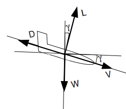
• a path angle [minus gamma] (that is the angle between ground level and aircraft trajectory, see Figure below);
• an aerodynamic speed V;
• and two acting external forces: the weight W and the aerodynamic force R, which we can consider resultant from lifting L and drag D.

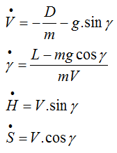
Using Newton's second law and proper treatment of reference coordinate systems, flight mechanics of gliding flight can be summarized by differential equation system below:



where m is the aircraft mass, g is the gravitational acceleration, W=mg, H is the height, S the range (distance from position in t=0) and dot over variables means time rate (derivative).

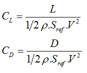
Before we can simulate gliding flight, one last note to take into consideration is that in Aeronautical Engineering we don't use lift and drag forces directly as project parameters. Instead we consider the following dimensionless coefficients:


where Sref is a reference area (in this case, wing area) and rho is the air density.

These parameters makes simpler the quantitative study of flight. Simulations of small-scale models in wind tunnels, for example, are just possible because of the called dynamic similarity enabled by dimensionless parameters approach. This means that a given state of flight in full-scale model can be reproduced in wind tunnel for small-scale model, allowing aircraft project improvements and saving costs.

Let's simulate!
This author strongly recommend the reader to try this simulation even if you are not familiar with scientific software. As you can see below, the codes are not hard to understand and the software uses a very high level programming language.

To solve the ordinary differential equation system above and simulate gliding flight, we're going to use Scilab, an open-source platform for numerical computation. If you don't have Scilab installed yet, download it and let's start programming.

Create a folder in your system, where you're going to put your scilab modules. In my Ubuntu (all the following pieces of information are valid for Windows too) my workplace is going to be /home/andre/doc/blog/gliding/scilab . Then, in Scilab console (the window showed when you open up the program), I change current directory, doing:

chdir('/home/andre/doc/blog/gliding/scilab')

for Windows, something like:

chdir('C:\Users\Andre\Documents\Blog\gliding\scilab')

In atmospherical flight, first step for simulation is an atmospherical model, i.e, for our purpose, functions for density and temperature calculation using height as input. Our model is ISA atmosphere. For now, just accept it.

In toolbar, click Launch Scipad button (the left first one) to create a new scilab model: our temperature function.

function T = temperature(H)
  T0 = 288.15; // Kelvin
  H0 = 0;
  g0 = 9.80665;
  L = -6.5e-3;
  if H <= 11000
    T = T0 + L*(H-H0);
  else
    T = temperature(11000);
  end
endfunction

This function just consider the first atmosphere layer (troposphere) presenting a linear gradient of temperature according to height. Save this file as temperature.sci . Create a new file for density function, copy the code below and save it as density.sci .

function rho = density(H)
  H0 = 0;
  g0 = 9.80665;
  R = 287.05287;
  T0 = 288.15;
  rho0 = 1.225;
  L = -6.5e-3;
  if H <= 11000
    rho = rho0*(temperature(H)/T0)^-(1+g0/(R*L));
  else
    rho = density(11000)*exp(-g0*(H-11000)/(R*temperature(11000)));
  end
endfunction

For now, don't care about redundancies in the codes above (for example, constants as g0). We are making so for simplicity. In further posts, we are going to improve the quality of code.

Now, the heart of simulation: the function for flight dynamics. Our approach here is to solve numerically the ordinary differential equation system (ODES) above, obtaining the state variables (V, gamma, H and S) in a given time t. To be solved by Scilab, one ODES has to be modeled by one function with input arguments being t and a vector X with state variables, and returning another vector with the first derivatives of each input variable. Code below shows function for gliding dynamics. Again, create a new file and save it as glidingdynamic.sci.

function Xdot = glidingdynamic(t,X)
  global CD0 k wingarea m g0 CL
  V = X(1);
  gamma_ = X(2);
  H = X(3);
  S = X(4);
  
  rho = density(H);
  CD = CD0+k*CL^2;
  L = 0.5*rho*V^2*wingarea*CL;
  D = 0.5*rho*V^2*wingarea*CD;
  
  Vdot = (-D-m*g0*sin(gamma_))/m;
  gammadot = (L-m*g0*cos(gamma_))/(m*V);
  Hdot = V*sin(gamma_);
  Sdot = V*cos(gamma_);
  Xdot = [ Vdot
       gammadot
       Hdot
       Sdot];
endfunction

Some comments about this code:

• Command global declares variables defined outside the scope of this function, i.e., these variables are going to be specified in another piece of code;


• X is a vector and in the first lines of the function, we just get the values of this vector, separatedly;


• gamma got a suffixed underline character ('_') for avoiding name conflict with a native scilab function called gamma;


• Drag coefficient (CD) is calculated for a kind of equation called Drag Polar, a function of CL;

Finally, let's instantiate the problem with a real glider parameters (wing area, mass, etc) and solve the system. In a new file, which we called gliding.sci we wrote the code below. This code is not a function, it is just a script (a sequence of scilab commands). See comments in the code (lines beginning with '//')

//globals variables that are going to be used
//by glidingdynamic function
global CD0 k wingarea m g0 CL

//loading all functions
exec('temperature.sci');
exec('density.sci');
exec('glidingdynamic.sci');

//specifying global parameters
//for more information about
//these aerodynamic parameters
//google about lift-induced drag
CD0 = 0.0115;
e = 0.94;
taperratio = 17;
k = 1/(%pi*taperratio*e);
wingarea = 16.01;
m = 512;
g0 = 9.80665;
CL = 0.75;

//some initial values for
//solve ODES
t0 = 0;
tf = 500;
V0 = 30; gamma0 = -5*%pi/180; H0 = 600; S0 = 0;
X0 = [ V0 gamma0 H0 S0 ];

//this creates a vector of time
//for solution: [0 0.01 0.02 ... 500]
t = t0:0.01:tf;

//this solves differential equation system
X = ode(X0,t0,t,glidingdynamic);

//next lines just slice solution vector X
//and plot graphs
Xdim = size(X);
i = 3:4:Xdim(2);
j = 4:4:Xdim(2);
plot(t,X(i)), xlabel('t(s)'), ylabel('H(m)')
figure
plot(X(j),X(i)), xlabel('S(m)'), ylabel('H(m)')

Further comments about the code:

• ode scilab function is the differential equation system solver. See scilab help for understanding its syntax.


• The last lines what we do it's just slicing the vector properly for plotting the desirable variables.

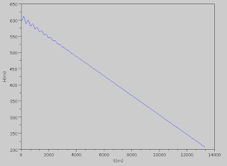
Figure below shows the trajectory of the glider in the first 500 seconds (time interval we chose for integration of motion equations).



In this simulation, one of our assumptions was constant value of CL during all the flight. In real situation, CL varies with angle of attack, which is modified by pilot's control to nose up or pitch down the aircraft. What if we could improve our code to let user change CL value during differential equation solving? This could be a dummy flight simulator. That's what we are going to do soon.