Tuesday, July 27, 2010

Dummy Gliding Simulator with Python

As we shown in previous post, gliding flight mechanics can be easily modeled and simulated. At that post, we used Scilab for solving dynamic system for a determined range of time and with constant lifting coefficient (CL). This time we are going to improve code using Python, flavoring simulation with PyGame and giving a dummy control to user.

Let's start preparing software platform for building our dummy flight simulator:

  • Python is a very powerful and clear programming language. If you have programmed before, you'll have no problem for understanding python codes;

  • SciPy is Python library for scientific programming. It is necessary download NumPy and, actual, SciPy;

  • PyGame "is a set of Python modules designed for writing games".
All these tools are available for both Linux and Windows users. Once you have installed these required software, the following instructions are valid independently of your operating system.

Designing code

Using Python, which has a different purpose than pure scientific tools as Scilab, we got more flexibility to modularize code and to make it become more reusable for future improvements.

So we are going to design our simulator with object oriented programming (OOP). If you are not familiar with this paradigm, we are going to give a very simple explanation that will hopefully become more clear with the codes written later.

OOP can be understood as a way to crack your code in little modules called classes, which are recipes for keeping together a set of data and a set of functions that change these data. Semantically, when modeling a problem, we bound the entities of the problem in classes, giving to them attributes and methods, i.e. actions that can change the entities behavior.

OK! Let's stop being abstract. See our physics model for gliding. We can identify an entity for Atmosphere stuff. So we can create the class Atmosphere with attributes about the values of temperature and density, for example; and with methods for changing temperature and density according height. Another class could be Aircraft with attributes like position and velocity, and methods to increase or decrease CL (this would be equivalent to give control to make aircraft to go up or to go down).

We call object, an individual of a given class. In other words, class is a recipe to build an object. For example, since we have an Aircraft class, we could create two different objects depending on values of their attributes, different polar drag, for instance.

Our model will contain the following main classes: Atmosphere, Aircraft and Flight.

Atmosphere class

For simplicity we're going to put all our code in just one python module (.py file extension). So, choose your favorite text editor and start putting the following code:


#!/usr/bin/python
# -*- coding: utf-8 -*-

from math import exp

class Atmosphere(object):
    T0 = 288.15
    H0 = 0
    g0 = 9.80665
    L = -6.5e-3
    R = 287.05287
    rho0 = 1.225
    
    def temperature(self,H):
        T = self.T0
        if H<=11000:
            T = self.T0 + self.L*(H-self.H0)
        else:
            T = self.temperature(11000)
        return T

    def density(self,H):
        rho = self.rho0
        if H<=11000:
            rho = self.rho0*(self.temperature(H)/self.T0)\
                  **(-(1+self.g0/(self.R*self.L)))
        else:
            rho = self.density(11000)*exp(-self.g0*\
                  (H-11000)/(self.R*self.temperature(11000)))
        return rho


Two initial lines are just some conventions and they can be even neglected for our purposes. Then we import exponential function (exp) from math library. Finally, we start code Atmosphere class. See that this code is very similar to Scilab code, but this time we have unified all atmospheric stuff in just one code structure, the class. Realize that methods are declared with def keyword and for accessing attribute values we have to use self identifier.

To test the code you can save the module as gliding.py and call it by command line:


$ python -i gliding.py 
>>> a = Atmosphere()
>>> a.density(600)
1.1559768882668726
>>> a.temperature(600)
284.25


In this test you are creating an object a from Atmosphere class and calling its methods density and, after, temperature for calculating these measures at height 600m.

Aircraft class

Now, the entity Aircraft. We should put CL and CD as methods, receiving angle of attack as parameter, but for our gliding flight we're going to consider constant CL or to change it directly. In other words, in real aircrafts, pilot got control over aerodynamic surfaces to change angle of attack. That changes CL. Here, we're going to make user (pilot) change CL value, directly, i.e. CL will be our control. To make it, we put an attribute CL_constant. Below it is the code you can append to previous code.


import math

class Aircraft(object):
    
    CD0 = 0
    taper_ratio = 0
    aspect_ratio = 0
    wing_area = 0
    mass = 0
    k = 0
    CL_constant = 1.0
    
    def __init__(self, CD0, taper_ratio, aspect_ratio, wing_area, mass):
        self.CD0 = CD0
        self.taper_ratio = taper_ratio
        self.aspect_ratio = aspect_ratio
        self.wing_area = wing_area
        self.mass = mass
        self.k = 1/(math.pi*aspect_ratio*taper_ratio);
        
    def CD(self,alfa=0.0):
        return self.CD0+self.k*self.CL(alfa)**2
    
    def CL(self,alfa=0.0):
        return self.CL_constant


Testing the code in python interpreter:

$ python -i gliding.py 
>>> a = Aircraft(CD0=0.0115, taper_ratio=0.94, \
                 aspect_ratio=17, wing_area=16.01, mass=512)
>>> a.CL()
1.0
>>> a.CD()
0.031419266970199665
>>> a.CL_constant = 1.5
>>> a.CL()
1.5
>>> a.CD()
0.056318350682949242


Flight class

This class uses some more specific object concepts as inheritance and composition. One class can inherits behavior from another class so that this subclass got the same methods of your superclass and, possibly, further methods. In our case, we have created a big class called Flight which can be reusable for many different kind of flights with different differential equation systems (ODES) modeling it. In Python you specify superclass for your class in parentheses following class name in class declaration. All previous classes inherits from object class (here you can see the reason for that). FlightSail class below inherits from Flight.

Flight class got methods for solving ODES, using SciPy library. We solve ODES by time slicing (says 1 second slice) and store ODES solution in a vector called state_history containing tuples in the form (t,y) where y is the vector representing one state of flight. In gliding flight y contains velocity, height, range, etc. Below we can see both classes Flight and subclass FlightSail.


import math
from scipy.integrate import ode
from scipy.integrate import odeint
from scipy.optimize import fsolve

class Flight(object):
    """Subclass this class and implement mech_ode_sys method
    """
    
    aircraft = None
    atmosphere = None
    
    def __init__(self,aircraft,atmosphere):
        self.aircraft = aircraft
        self.atmosphere = atmosphere
        
    def mech_ode_sys(self, t, state):
        """Must be implemented by subclass
        """    
    
    def start(self, initial_state, t_0 = 0, dt = 1):
        self.ode_solver = ode(self.mech_ode_sys).set_integrator('vode')
        self.ode_solver.set_initial_value(initial_state, t_0)
        self.dt = dt
        self.state_history = [[0.0,initial_state]]
    
    def next_state(self):
        if self.ode_solver.successful():
            self.ode_solver.integrate(self.ode_solver.t+self.dt)
            self.state_history.append((self.ode_solver.t, self.ode_solver.y,))
            return [self.ode_solver.t, self.ode_solver.y]
        else:
            return None
    
    def solve(self,t):
        """Solve ODE system for a given array of values t
        """
        def func(state,t):
            return self.mech_ode_sys(t, state)
        
        y0 = self.state_history[-1][1]
        y = odeint(func,y0,t)
        states = zip(t,y[:])
        self.state_history += states 
        return states

class FlightSail(Flight):
    
    VELOCITY = 0
    GAMMA = 1
    HEIGHT = 2
    RANGE = 3
    
    def __init__(self,aircraft,atmosphere):
        super(FlightSail,self).__init__(aircraft,atmosphere)
        
    def mech_ode_sys(self, t, state):
        """state is a tuple in the form (Velocity,gamma,Height,Range)
        """
        V = state[VELOCITY]
        gamma = state[GAMMA]
        H = state[HEIGHT]
        R = state[RANGE]
        
        CL = self.aircraft.CL()
        CD = self.aircraft.CD()
        m = self.aircraft.mass
        
        rho = self.atmosphere.rho(H)
        
        A = self.aircraft.wing_area
        
        L = 0.5*rho*V**2*A*CL
        D = 0.5*rho*V**2*A*CD
        
        V_p = (-D-m*self.atmosphere.g_0*math.sin(gamma))/m
        gamma_p = (L-m*self.atmosphere.g_0*math.cos(gamma))/(m*V)
        H_p = V*math.sin(gamma)
        R_p = V*math.cos(gamma)
        return [V_p, gamma_p, H_p, R_p]


Putting it all together

Now, instantiating the same problem from previous post.


import math

atmosphere = Atmosphere()
a = Aircraft(CD0=0.0115, taper_ratio=0.94, \
             aspect_ratio=17, wing_area=16.01, mass=512)
a.CL_constant = 0.75
sail = FlightSail(aircraft=a, atmosphere=atmosphere)
V_0 = 30
gamma_0 = -3*math.pi/180
H_0 = 600
R_0 = 0
state_0 = (V_0, gamma_0, H_0, R_0)
sail.start(initial_state=state_0)
aircraft_state = list(state_0)
MAX_RANGE = 14000


For using PyGame we have put a profile aircraft figure (in our case Super Tucano) and just update its position in a 640 x 480 screen, let CL ranging according up and down keys, and adjusting path angle, rotating the figure (this is not correct, but we are neglecting angle of attack here). PyGame code is shown below:


pygame.init()
SCREEN_X_MAX = 640
SCREEN_Y_MAX = 480
screen = pygame.display.set_mode((SCREEN_X_MAX,SCREEN_Y_MAX))
tucano_img_original = pygame.image.\
                        load('supertucano_lateral_menor.bmp').convert()

pygame.display.update()
tucano_img = None 
clock = pygame.time.Clock()
clock.tick(10)
start = False

while True:
    for event in pygame.event.get():
        if event.type == pygame.QUIT:
            sys.exit()
        elif event.type == pygame.KEYDOWN:
            start = True
    
    key = pygame.key.get_pressed()
    if key[pygame.K_UP]:
        sail.aircraft.CL_constant += 0.1
        print "CL increasing to: "+str(sail.aircraft.CL_constant)
    elif key[pygame.K_DOWN]:
        sail.aircraft.CL_constant -= 0.1
        print "CL decreasing to: "+str(sail.aircraft.CL_constant)
    
    if start:
        state = sail.next_state()
        #print state
        pygame.display.set_caption('Sail Flight t = '+str(state[0]))
        aircraft_state = [i for i in state[1]]
        x = aircraft_state[FlightSail.RANGE]/float(MAX_RANGE)\
                         *SCREEN_X_MAX
        y = SCREEN_Y_MAX - float(aircraft_state[FlightSail.HEIGHT])\
                         /H_0*SCREEN_Y_MAX
        tucano_img = pygame.transform.rotate(tucano_img_original,\
                         aircraft_state[FlightSail.GAMMA]/math.pi*180)
        screen.fill((255,255,255))
        screen.blit(tucano_img,(x,y))
        pygame.display.update()
        pygame.time.delay(100)


Figure below shows whole code running (using python gliding.py at command line).


And that is it! Keys UP and DOWN changes CL directly, what is not quiet representative but it is fun though.
Wednesday, July 21, 2010

Gliding Flight Mechanics

Gliding is an unpowered flight of an aircraft. Gliders, or sailplanes, are the aircrafts designed for gliding flight. Since they don't have any engine for propulsion to takeoff, they need alternative methods to get airborne. These methods include aerotowing and winch launching. For the former, the glider takeoff attached with a powered plane by a tow rope. Once they get a desirable height, tow-rope is released. By winch launching, glider uses a grounded-base winch (mounted on a heavy vehicle) to be launched up to 700 m after a short, steep ride. There are others possible launch methods for gliders.

But gliding flights are not exclusive for gliders. Jet transport aircrafts are better gliders than people can think. If things go really bad during flight and the plane loses all engines, it can glide and land safely. A famous example was the nicknamed Gimli Glider. An aviation incident involving the Air Canada Boeing 767-200, which flew "completely out of fuel at 7,920 m about halfway through your flight from Montreal to Edmonton via Otawa". "None of 61 passengers were seriously hurt".

We can study flight mechanics of gliding, supported by basic Physics, eventhough with good approximations. Before considering free body diagram of aircraft, let us note that there is a force in the airplane which makes it different of, says, a rock: the aerodynamic force. Geometrical shape of wings makes the flow (wind) pushes aircraft back (drag force) and pulls it up (lifting force), producing an amazing effect we call flying.

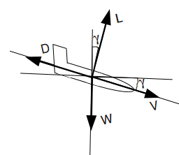
Suppose an aircraft gliding with:
  • a path angle [minus gamma] (that is the angle between ground level and aircraft trajectory, see Figure below);
  • an aerodynamic speed V;
  • and two acting external forces: the weight W and the aerodynamic force R, which we can consider resultant from lifting L and drag D.
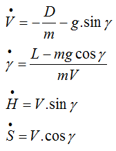
Using Newton's second law and proper treatment of reference coordinate systems, flight mechanics of gliding flight can be summarized by differential equation system below:


where m is the aircraft mass, g is the gravitational acceleration, W=mg, H is the height, S the range (distance from position in t=0) and dot over variables means time rate (derivative).

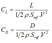
Before we can simulate gliding flight, one last note to take into consideration is that in Aeronautical Engineering we don't use lift and drag forces directly as project parameters. Instead we consider the following dimensionless coefficients:


where Sref is a reference area (in this case, wing area) and rho is the air density.

These parameters makes simpler the quantitative study of flight. Simulations of small-scale models in wind tunnels, for example, are just possible because of the called dynamic similarity enabled by dimensionless parameters approach. This means that a given state of flight in full-scale model can be reproduced in wind tunnel for small-scale model, allowing aircraft project improvements and saving costs.

Let's simulate!
This author strongly recommend the reader to try this simulation even if you are not familiar with scientific software. As you can see below, the codes are not hard to understand and the software uses a very high level programming language.

To solve
the ordinary differential equation system above and simulate gliding flight, we're going to use Scilab, an open-source platform for numerical computation. If you don't have Scilab installed yet, download it and let's start programming.

Create a folder in your system, where you're going to put your scilab modules. In my Ubuntu (all the following pieces of information are valid for Windows too) my workplace is going to be /home/andre/doc/blog/gliding/scilab . Then, in Scilab console (the window showed when you open up the program), I change current directory, doing:


chdir('/home/andre/doc/blog/gliding/scilab')


for Windows, something like:


chdir('C:\Users\Andre\Documents\Blog\gliding\scilab')


In atmospherical flight, first step for simulation is an atmospherical model, i.e, for our purpose, functions for density and temperature calculation using height as input. Our model is ISA atmosphere. For now, just accept it.

In toolbar, click Launch Scipad button (the left first one) to create a new scilab model: our temperature function.


function T = temperature(H)
  T0 = 288.15; // Kelvin
  H0 = 0;
  g0 = 9.80665;
  L = -6.5e-3;
  if H <= 11000
    T = T0 + L*(H-H0);
  else
    T = temperature(11000);
  end
endfunction


This function just consider the first atmosphere layer (troposphere) presenting a linear gradient of temperature according to height. Save this file as temperature.sci . Create a new file for density function, copy the code below and save it as density.sci .


function rho = density(H)
  H0 = 0;
  g0 = 9.80665;
  R = 287.05287;
  T0 = 288.15;
  rho0 = 1.225;
  L = -6.5e-3;
  if H <= 11000
    rho = rho0*(temperature(H)/T0)^-(1+g0/(R*L));
  else
    rho = density(11000)*exp(-g0*(H-11000)/(R*temperature(11000)));
  end
endfunction


For now, don't care about redundancies in the codes above (for example, constants as g0). We are making so for simplicity. In further posts, we are going to improve the quality of code.

Now, the heart of simulation: the function for flight dynamics. Our approach here is to solve numerically the ordinary differential equation system (ODES) above, obtaining the state variables (V, gamma, H and S) in a given time t. To be solved by Scilab, one ODES has to be modeled by one function with input arguments being t and a vector X with state variables, and returning another vector with the first derivatives of each input variable. Code below shows function for gliding dynamics. Again, create a new file and save it as glidingdynamic.sci.


function Xdot = glidingdynamic(t,X)
  global CD0 k wingarea m g0 CL
  V = X(1);
  gamma_ = X(2);
  H = X(3);
  S = X(4);
  
  rho = density(H);
  CD = CD0+k*CL^2;
  L = 0.5*rho*V^2*wingarea*CL;
  D = 0.5*rho*V^2*wingarea*CD;
  
  Vdot = (-D-m*g0*sin(gamma_))/m;
  gammadot = (L-m*g0*cos(gamma_))/(m*V);
  Hdot = V*sin(gamma_);
  Sdot = V*cos(gamma_);
  Xdot = [ Vdot
       gammadot
       Hdot
       Sdot];
endfunction


Some comments about this code:

  • Command global declares variables defined outside the scope of this function, i.e., these variables are going to be specified in another piece of code;

  • X is a vector and in the first lines of the function, we just get the values of this vector, separatedly;

  • gamma got a suffixed underline character ('_') for avoiding name conflict with a native scilab function called gamma;

  • Drag coefficient (CD) is calculated for a kind of equation called Drag Polar, a function of CL;


Finally, let's instantiate the problem with a real glider parameters (wing area, mass, etc) and solve the system. In a new file, which we called gliding.sci we wrote the code below. This code is not a function, it is just a script (a sequence of scilab commands). See comments in the code (lines beginning with '//')

//globals variables that are going to be used
//by glidingdynamic function
global CD0 k wingarea m g0 CL

//loading all functions
exec('temperature.sci');
exec('density.sci');
exec('glidingdynamic.sci');

//specifying global parameters
//for more information about
//these aerodynamic parameters
//google about lift-induced drag
CD0 = 0.0115;
e = 0.94;
taperratio = 17;
k = 1/(%pi*taperratio*e);
wingarea = 16.01;
m = 512;
g0 = 9.80665;
CL = 0.75;

//some initial values for
//solve ODES
t0 = 0;
tf = 500;
V0 = 30; gamma0 = -5*%pi/180; H0 = 600; S0 = 0;
X0 = [ V0 gamma0 H0 S0 ];

//this creates a vector of time
//for solution: [0 0.01 0.02 ... 500]
t = t0:0.01:tf;

//this solves differential equation system
X = ode(X0,t0,t,glidingdynamic);

//next lines just slice solution vector X
//and plot graphs
Xdim = size(X);
i = 3:4:Xdim(2);
j = 4:4:Xdim(2);
plot(t,X(i)), xlabel('t(s)'), ylabel('H(m)')
figure
plot(X(j),X(i)), xlabel('S(m)'), ylabel('H(m)')


Further comments about the code:

  • ode scilab function is the differential equation system solver. See scilab help for understanding its syntax.

  • The last lines what we do it's just slicing the vector properly for plotting the desirable variables.

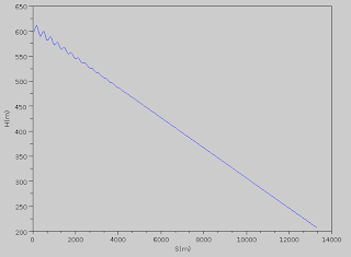
Figure below shows the trajectory of the glider in the first 500 seconds (time interval we chose for integration of motion equations).


In this simulation, one of our assumptions was constant value of CL during all the flight. In real situation, CL varies with angle of attack, which is modified by pilot's control to nose up or pitch down the aircraft. What if we could improve our code to let user change CL value during differential equation solving? This could be a dummy flight simulator. That's what we are going to do soon.